Technical Information SAXS/WAXS
- SAXS Cluster (Unlicensed)

This page details the technical specifications and development of the SAXS beamline. For information about running samples please refer to the Beamline wiki .
Commissioning of the beamline optics was completed in 2009 and the full range of energies and camera lengths is available with the beamline running a full operations program since mid-2009. Development of the endstation has provided rapid & reliable methods for video camera based sample alignment and a flexible sample stage allows straightforward sample mounting. Sample mounting is continuing to be developed on the beamline with a focus on improved efficiency and higher sample throughput.
Two Pilatus detectors are in operation for SAXS (2M detector) and WAXS (100k detector) and may be run concurrently with excellent dynamic range, low noise and short exposures with up to 30 and 150 frames per second.
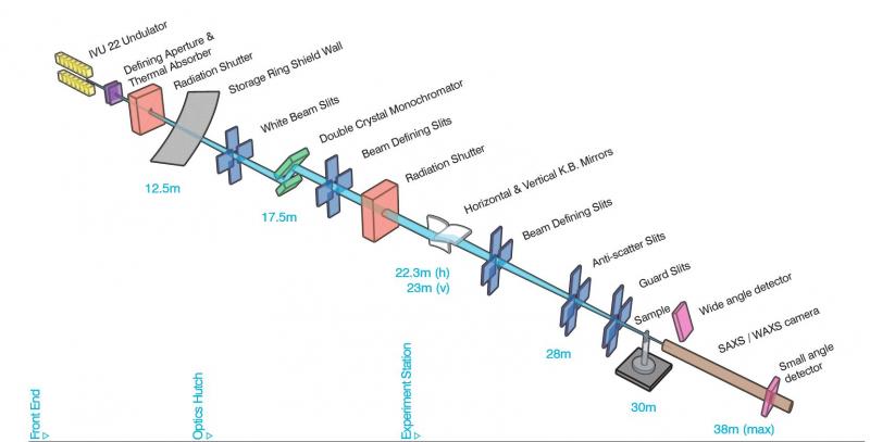
Schematic Diagram of the SAXS /WAXS Beamline
Technical Specifications
Source | In-vacuum undulator, 22 mm period, 3 m length, Kmax 1.56 |
|---|---|
Energy range | 5.5 - 21 keV. Optimised for 8.15 keV and 11.5 keV. |
Energy resolution | 2 x 10⁻⁴ from cryo-cooled Si(111) double crystal monochromator. |
Mirrors | Horizontal and vertical focusing mirrors for monochromatic beam, typically focused at the sample position. Either or both mirrors may be removed for specialty experiments. Solution scattering is typically done without vertical focusing. Mirror stripes (Si, Rh) allow full coverage of energy range rejecting higher energy harmonics. |
Maximum flux at sample | 2 x 10¹³ photons per second at 8 keV. 8 x 10¹² photons per second at 11.5 keV. |
Beam size at sample (sample position focus) | 250 µm horizontal × 25 µm vertical (FWHM) 250 µm horizontal × 450 µm vertical (FWHM, unfocused vertical for solution scattering) 1000 µm horizontal × 450 µm vertical (FWHM, unfocused) |
Beam divergence at sample position | 140-260 µrad horizontal 30 - 60 µrad vertical depending on focal position. |
q-range | SAXS - 0.0015 - 3.0 Å-1 (using 2+ camera lengths between ~500 and 7400 mm) SAXS detector in vacuum and fully motorized for automated camera length changes WAXS - 0.6 - 5 Å-1 (energy dependent) |
Instrument background (assuming 1mm sample pathlength) | In-air samples: background < 0.02 cm-1 @ q=0.01 Å-1 In-vacuum samples: background < 0.00001 cm-1 @ q=0.01 Å-1 |
Q-range & SAXS Camera Lengths
Q-ranges are calculated for a 12 keV beam (1.0322 Å wavelength). These scattering angle ranges may be further adjusted by selecting different beam energies (5.2 - 21 keV) or by slightly modifying the camera length by attaching longer or shorter nosecones as in the interactive q calculator for different SAXS camera setups. The Q-range and camera setup required for an experiment must be included in applications for beam time. If additional information is required please contact beamline staff.
Camera length (mm) | Design | Q-range (Å-1) at 12 keV | D spacing range (Å) at 12 keV | Extension tube | Nosecone |
|---|---|---|---|---|---|
550 | Shortest | Stumpy | 0.03 – 1.30 | 5 – 227 | |
700 | Short | 0.02 – 1.03 | 6 – 289 | ||
940 | Long | 0.02 – 0.77 | 8 – 389 | ||
1000 | Offset | 0.02 – 0.73 | 9 – 413 | ||
1280 | Short | Short | 0.01 – 0.57 | 11 – 529 | |
1426 | Protein | 0.01 – 0.51 | 12 – 589 | ||
1520 | Long | 0.01 – 0.48 | 13 – 628 | ||
1580 | Offset | 0.01 – 0.46 | 14 – 653 | ||
2680 | Medium | Protein* | 0.005 – 0.27 | 23 – 1108 | |
3120 | Short + Medium | Short | 0.004 – 0.24 | 27 – 1290 | |
3256 | Protein | 0.004 – 0.22 | 28 – 1346 | ||
3350 | Long | 0.004 – 0.22 | 29 – 1385 | ||
3410 | Offset | 0.004 – 0.21 | 29 – 1409 | ||
7040 | Short + Medium + Long | Short | 0.002 – 0.10 | 61 – 2910 | |
7160 | Protein | 0.002 – 0.10 | 62 – 2959 | ||
7270 | Long | 0.002 – 0.10 | 63 – 3005 | ||
7330 | Offset | 0.002 – 0.10 | 63 – 3030 |
*- recommended for most proteins
Instrument Background
The beamline is well suited to analysing weakly scattering samples due to high flux and low parasitic scattering. An in vacuum sample chamber is available for particularly weak scattering samples, either in transmission or grazing incidence geometries.
How weak a scatterer can be analysed?
Below is the measured background intensity at two main camera lengths calibrated into absolute intensity units (assuming a 1.0 mm sample thickness), for samples either measured in air or in vacuum.
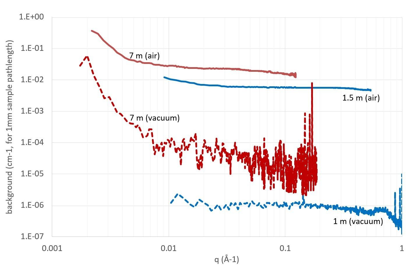
For measurement in air, the instrument background is controlled by air scattering above approximately 0.01Å-1 . Below approximately 0.01 Å-1, the instrument background is controlled mostly by the instrument itself, primarily by weak scattering from the silicon nitride vacuum windows either side of the sample. . There is a good chance of getting usable data if the net scattering (sample minus background) is a few percent above the instrument background.
For in-vacuum measurement, all sources of background have been controlled and there is almost no background intensity above ~ 0.005 Å-1, especially for camera lengths under 3 m. Below ~ 0.005 Å-1 the instrument background currently rises due to parasitic scattering from the beamline optics, ultimately because of figure errors on the HFM which can only be partially removed by the beamline’s slit system. The instrument background between 0.0015 - 0.004 Å-1 would only affect the weakest of scattering solid samples run in vacuum, whose mount or containment itself does not cause any scattering. In the case of proteins, scattering from the capillary and the solvent typically dominate the measurement, not the instrument background.
For weakly scattering samples, it may be worth doing some planning calculations to check whether the scattering is likely to be observable. The main thing to know is how much background will come from your sample mounting system, as this usually dominates over the instrument background. A signal:noise of ~1.02 (i.e. only 2% signal) is usually measurable given the accuracy of normalisation is well below 0.1% (depending on transmitted flux). Some general suggestions are:
samples run in capillaries, or between tapes like Kapton: the background will be controlled by your sample cell, mount or solvent, not the optics
For water based solutions (e.g. proteins) the background will be controlled mostly by the cell below ~0.02 cm-1, and at higher q by the solvent (note: water scattering intensity is = 0.0163 cm-1).
the vacuum in the sample chamber is below 1 x 10⁻⁵ mbar. Your samples will need to be compatible with low vacuum.
for in-vacuum grazing incidence WAXS, the instrument background is so low that sub-monolayer GIWAXS has been done on crystalline polymer films.
Beamline Flux
The beamline is capable of utilising x-rays in the range of 5.5 - 21 keV with the optics optimised for the 8 - 12 keV range. The flux delivered at the sample position is dependent upon the undulator harmonic selected as shown below for the 5th and 7th harmonics. The 3rd, 5th, 7th, 9th and 11th harmonics may be selected to cover the full energy range with somewhat lower flux delivered for higher harmonics and higher energies.
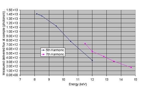
Flux at the sample position for 5th and 7th undulator harmonics
Detector Specifications
The SAXS beamline uses two Pilatus3 detectors for SAXS (2M, 254 mm x 289 mm) and WAXS (100k, 33 mm x 84 mm) data collection. The detectors are in-vacuum and fully motorised, for fast, automated changes of configuration (e.g. SAXS camera length).
The large area SAXS detector provides excellent 2D data collection for SAXS and 2D WAXS collection. The small WAXS detector can be used for simultaneous SAXS/WAXS experiments, or for fast time resolved experiments (>25 frames/second) when required. Whilst the dedicated WAXS detector adds value in those limited cases, most WAXS experiments are performed using the much larger SAXS detector brought to the sample for maximum sensitivity and angular range.
Time-resolved data collection is also well supported as the Pilatus detectors are capable of collection at 25 Hz (2M) and 500 Hz (100K).
Detector | Specifications |
|---|---|
Dectris - Pilatus3-2M (In-vacuum) |
|
Dectris - Pilatus3-100K (In-vacuum) |
|